Understanding the relationship between flow rate and the hydraulic resistance your pump must overcome
When selecting or evaluating a pump for any piping system, one of the most fundamental tools at your disposal is the System Curve. It describes, for every possible flow rate, exactly how much head the system demands — a number shaped by elevation changes, pipe geometry, fluid properties, and friction. Overlay it with a pump’s performance curve, and the intersection tells you precisely where your system will operate.
This post walks through the full derivation, step by step.
What Is the System Curve?
The System Curve maps flow rate Q to the total head H_{\text{system}} required to move fluid through the system at that rate. It is not a property of the pump — it is a property of the pipes, fittings, elevations, and fluid in your installation.
Its governing equation is elegantly simple:
H_{\text{system}} = H_{\text{static}} + \Delta hTwo components. One fixed, one variable. Let’s unpack both.
Step 1 — Static Head
H_{\text{static}} is the elevation difference the pump must overcome regardless of how fast fluid is moving. It is purely a function of geometry:
H_{\text{static}} = z_{\text{outlet}} - z_{\text{inlet}}If your outlet is 5 m above your inlet, the pump must supply at least 5 m of head just to lift the fluid — before a single joule is lost to friction. If the outlet is below the inlet, static head is negative, and gravity actually assists the flow.
Step 2 — Friction Head Loss
\Delta h is where it gets interesting. This term captures all energy lost to friction as fluid travels through the pipe, and it grows with flow rate. To calculate it, we use the Darcy-Weisbach equation:
\Delta h = f \cdot \frac{L v^{2}}{2 g D}| Symbol | Meaning | Unit |
|---|---|---|
| f | Darcy friction factor | — |
| L | Pipe length | m |
| v | Flow velocity | m/s |
| g | Gravitational acceleration (9.81) | m/s² |
| D | Pipe inner diameter | m |
| \Delta h | Head loss due to friction | m |
Notice that \Delta h scales with v^{2} — double the velocity and friction loss quadruples. This is why the System Curve takes its characteristic parabolic shape.
To evaluate this equation, we need three things: the velocity v, the friction factor f, and both require a little more work.
Step 3 — Velocity from Flow Rate
Velocity is not an independent input — it follows directly from the flow rate Q and the pipe’s cross-sectional area A, via the continuity equation:
v = \frac{Q}{A}And the area of a circular pipe is simply:
A = \pi \left(\frac{D}{2}\right)^{2}So for any chosen flow rate Q and known pipe diameter D, velocity is fully determined.
Step 4 — The Friction Factor
The Darcy friction factor f is the trickiest piece. It depends on how turbulent the flow is and how rough the pipe walls are. We calculate it in two stages.
4a — Reynolds Number
First, we establish the flow regime using the Reynolds number:
Re = \frac{\rho \, v \, D}{\mu}| Symbol | Meaning | Unit |
|---|---|---|
| \rho | Fluid density | kg/m³ |
| v | Flow velocity | m/s |
| D | Pipe diameter | m |
| \mu | Dynamic viscosity | Pa·s |
For water at 20 °C, \rho \approx 998 \; \text{kg/m}^{3} and \mu \approx 0.001 \; \text{Pa} \cdot \text{s}. Fluid density itself follows from first principles:
\rho = \frac{M}{V}where M is the mass of the fluid and V is its volume. For most engineering applications, tabulated values for your fluid and temperature are sufficient.
A Reynolds number below ~2300 indicates laminar flow; above ~4000 indicates fully turbulent flow. Most pump systems operate well into the turbulent regime.
4b — Swamee-Jain Approximation
With Re in hand, we can compute f directly — no iteration required — using the Swamee-Jain approximation:
f = \frac{0.25}{\left[ \log\left( \frac{\varepsilon / D}{3.7} + \frac{5.74}{Re^{\,0.9}} \right) \right]^{2}}| Symbol | Meaning | Unit |
|---|---|---|
| \varepsilon | Pipe roughness | m |
| D | Pipe diameter | m |
| Re | Reynolds number | — |
Typical roughness values: drawn copper or plastic pipe \varepsilon \approx 0.0000015 \; \text{m}; commercial steel \varepsilon \approx 0.000046 \; \text{m}; cast iron \varepsilon \approx 0.00026 \; \text{m}. The rougher the pipe, the higher f, and the steeper the System Curve climbs.
Putting It All Together
The calculation is a dependency chain that resolves from the bottom up:
Q → v = Q/A → Re = ρvD/μ → f (Swamee-Jain) → Δh (Darcy-Weisbach) → H_system
To build the full System Curve, repeat this chain for a range of flow rates — typically from Q = 0 up to the maximum flow your system might ever see. At Q = 0, friction vanishes and H_{\text{system}} = H_{\text{static}}. As Q increases, \Delta h grows as Q^{2}, tracing the parabola upward.
\boxed{ H_{\text{system}}(Q) = H_{\text{static}} + f(Q) \cdot \frac{L}{2 g D} \cdot \left(\frac{Q}{A}\right)^{2} }This single expression — once expanded with the Swamee-Jain friction factor — gives you the complete System Curve as a function of flow rate.
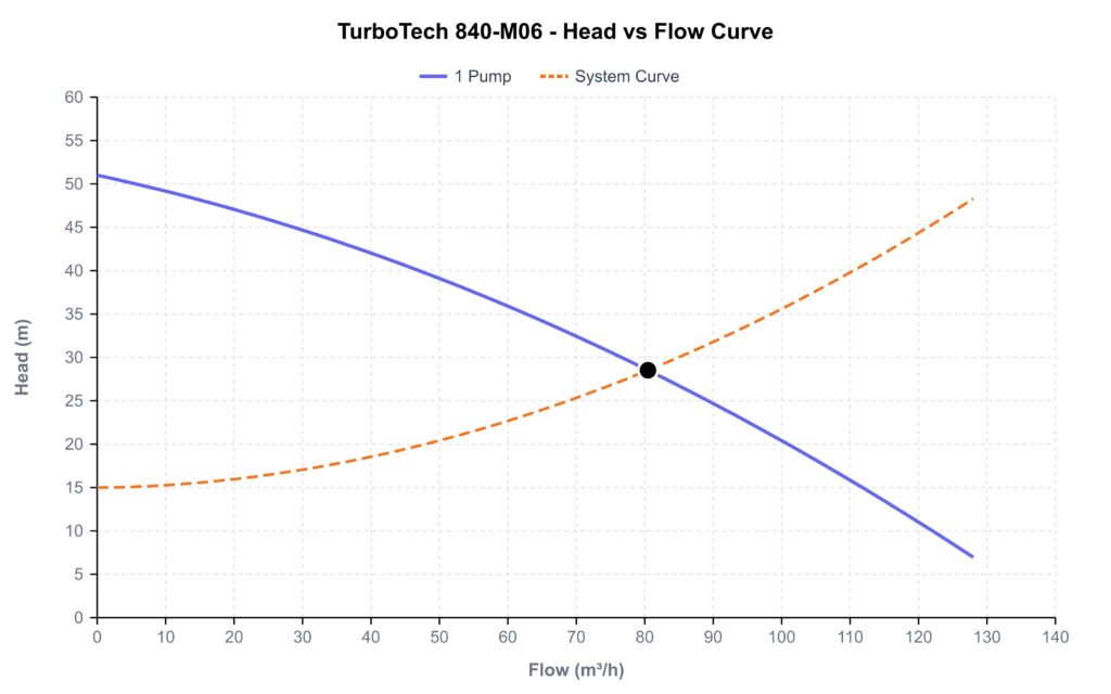
The Operating Point
The System Curve becomes most powerful when overlaid with a pump performance curve (also called the H-Q curve). The pump curve slopes downward — higher flow, lower delivered head. The System Curve slopes upward. Their intersection is the operating point: the flow rate and head at which the system will naturally settle.
If the operating point sits far from the pump’s best efficiency point (BEP), the installation is either oversized or undersized, wasting energy or failing to meet demand. Calculating the System Curve first is what makes an informed pump selection possible.
Skip the Spreadsheet
Working through this chain by hand — or in a spreadsheet you’ll have to rebuild for every project — is tedious and error-prone. A mistyped roughness value or a forgotten unit conversion is all it takes to land on the wrong pump.
digirom’s pump selection software handles all of this automatically — system curve calculation, performance curve overlay, operating point identification — giving your customers a seamless selection experience built into your product. Book a demo and we’ll show you exactly how to implement it for your catalogue.
Summary
The System Curve is built from two additive terms: a constant static head from elevation difference, and a flow-dependent friction loss that grows parabolically. Computing it requires working through a chain of hydraulic relationships:
- Convert flow rate to velocity using the continuity equation.
- Compute the Reynolds number from fluid properties and velocity.
- Use the Swamee-Jain equation to find the Darcy friction factor.
- Apply Darcy-Weisbach to calculate head loss.
- Add static head to obtain total system head.
Repeat across the full flow range and you have your System Curve — the essential foundation for any pump system analysis.